Pascal’s Mugging: Reasoning when you have other things to do

Epistemic status: I don’t think anything I’m saying in this post is completely new (eg see https://www.lesswrong.com/posts/Ap4KfkHyxjYPDiqh2/pascal-s-muggle-infinitesimal-priors-and-strong-evidence and https://www.gwern.net/mugging) apart from maybe the meta-probability framing, but it’s an exercise in writing my half-formed thoughts down and trying to explain them clearly.

This post has two parts. In the first I’ll try to pin down the rhetorical sleight of hand in Nick Bostrom article on Pascal’s Mugging, which confused me for a long time. In the second, I’ll muse about the question of how to reason about events that are both “huge if true” and “astronomically unlikely”, and argue with https://nintil.com/pascals-mugging/. In a later post I might analyse the Kolmogorov-complexity-theoretic issues that come up when you try to stop your favourite hard-coded logico-symbolic VNM maximising AI from spending all its time dreaming about winning the intergalactic lottery.

Part 1

Pascal’s Wager is a famous argument that “a rational person should live as though God exists and seek to believe in God. If God does not exist, such a person will have only a finite loss (some pleasures, luxury, etc.), whereas if God does exist, he stands to receive infinite gains (as represented by eternity in Heaven) and avoid infinite losses (an eternity in Hell).” Thus the expected value of praying with true faith is infinite and you should make sure to do it.

In Nick Bostrom’s whimsical article Pascal’s Mugging, Pascal gets asked for money by someone who claims they will use their magical powers to do great deeds of wonder and delight in return.

Pascal: It is possible that you have the magic powers that you claim to have,
but let me tell you, I give that a very, very low probability.
Mugger: That’s fine. But tell me, how low a probability exactly? Remember,
you might think it all seems implausible, but we are all fallible, right? And
you must admit, from what you’ve already seen and heard, that I am a rather
atypical mugger. And look at my pale countenance, my dark eyes; and note
that I’m dressed in black from top to toe. These are some of the telltale signs
of an Operator of the Seventh Dimension. That’s where I come from and
that’s where the magic work gets done.
Pascal: Gee . . . OK, don’t take this personally, but my credence that you have
these magic powers whereof you speak is about one in a quadrillion.
Mugger: Wow, you are pretty confident in your own ability to tell a liar from
an honest man! But no matter. Let me also ask you, what’s your probability
that I not only have magic powers but that I will also use them to deliver on
any promise – however extravagantly generous it may seem – that I might
make to you tonight?
Pascal: Well, if you really were an Operator from the Seventh Dimension as
you assert, then I suppose it’s not such a stretch to suppose that you might
also be right in this additional claim. So, I’d say one in 10 quadrillion.
Mugger: Good. Now we will do some maths. Let us say that the 10 livres that
you have in your wallet are worth to you the equivalent of one happy day.
Let’s call this quantity of good 1 Util. So I ask you to give up 1 Util. In return,
I could promise to perform the magic tomorrow that will give you an extra
10 quadrillion happy days, i.e. 10 quadrillion Utils. Since you say there is a 1
in 10 quadrillion probability that I will fulfil my promise, this would be a fair
deal. The expected Utility for you would be zero. But I feel generous this
evening, and I will make you a better deal: If you hand me your wallet, I will
perform magic that will give you an extra 1,000 quadrillion happy days
of life.
Pascal: I admit I see no flaw in your mathematics.
Mugger: This is my final offer. You’re not going to pass up a deal that we
have just calculated will give you an expected Utility surplus of nearly 100
Utils, are you? That’s the best offer you are likely to see this year.
Pascal: Is this legitimate? You know, I’ve committed myself to trying to be a
good Christian.
Mugger: Of course it’s legitimate! Think of it as foreign trade. Your currency
is worth a lot in the Seventh Dimension. By agreeing to this transaction, you
give a major boost to our economy. Oh, and did I mention the children?
If only you could see the faces of the sweet little orphans who will be made so
much better off if we get this influx of hard currency – and there are so many
of them, so very, very, very many … .
Pascal: I must confess: I’ve been having doubts about the mathematics of
infinity. Infinite values lead to many strange conclusions and paradoxes. You
know the reasoning that has come to be known as ‘Pascal’s Wager’? Between
you and me, some of the critiques I’ve seen have made me wonder whether I
might not be somehow confused about infinities or about the existence of
infinite values…
Mugger: I assure you, my powers are strictly finite. The offer before you does
not involve infinite values in any way.
https://nickbostrom.com/papers/pascal.pdf

Wikipedia claims (as of this posting): “The name refers to Pascal’s Wager, but unlike the wager, it does not require infinite rewards. This sidesteps many objections to the Pascal’s Wager dilemma that are based on the nature of infinity.”

Not infinite, huh? It depends on how you interpret the question “What’s your probability
that I not only have magic powers but that I will also use them to deliver on
ANY promise that I might
make to you tonight?”

Either we assume the mugger can give us X utils (the unit of rewards and desserts, whether just or offered out of the blue) for any possible X we name, and try to put a probability on this as a whole. But this means that the mugger possesses (or can give away) an amount of utility larger than any finite X – which brings us back to infinity again.

Part 2

Or we could think in terms of our prior probability being a function of X, and try to figure out what it is, and what to do (which are importantly different questions) AFTER the mugger names a number.

As it happens, the mugger saying stuff isn’t very important, because it doesn’t cost malicious nerdsnipers anything to claim they have magic powers.

Using Bayes Rule,

$P(reward | claim) = \frac{P(claim | power)}{(P(claim|power)*P(power) + P(claim | no \;power) * P(no \; power)} P(power)$

Since P(claim | no power) * P(no power) is pretty close to 1, the fraction is not much larger than 1, so the only thing that matters is your original belief in magic/the simulation argument P(power).

But this means that we might as well consider the muggers we might meet tomorrow, aka the ones in our head. As the blog Nintil puts it:

Consider the act of closing the document you are now reading. It is conceivable that a being in Dimension N will kill you if you do so, for not having a permanently open view of Nintil is sacrilegious. What’s the probability of that? Similarly, in dimension L, thinking that Nintil is not the best blog in the world is a hideous act, and is punished by death, even for us inhabitants of the regular universe. What’s the probability of that? Furthermore, should you close Nintil? Should you dare think Nintil is not the best blog ever?
https://nintil.com/pascals-mugging/#wrong

With just the prior probability, the expected utility framework tells you not to give the mugger anything as long as your prior decreases fast enough to make the infinite sums converge to something smaller than the total cost of paying the mugger. Gwern has an argument that if your prior falls off faster than inverse linear then the mugger can get around it by asking you for very small amounts repeatedly, but I think this ignores that the cost of paying the mugger includes transaction costs.

How does one deal with the general possibility of astronomically low probability events having very high impacts?

The natural answer is that beyond a certain point (which varies with one’s anxiety levels) one deals with them by ignoring them.

Note that I am NOT talking about X-risk scenarios ala The Precipice, which are not astronomically low prob but are in fact SCARY HIGH. When I say astronomically low I mean numbers like (1/10^10^10^10) etc.

Anyway, Jose (the author of Nintil) objects to the “ignore things” strategy with an opposing psychiatric diagnosis:

That it seems to condemn us to the epistemic version of bipolar disorder: We are believing that the probability of the mugger being from another dimension is nonzero, and at the same time we are acting as if it were zero.
https://nintil.com/pascals-mugging/#logical

But I think this is fine, and can be defended using a framework of metaprobabilities (eg Jaynes Ap) – see https://www.lesswrong.com/posts/2xmKZu73gZLDEQw7c/probability-knowledge-and-meta-probability for a discussion.

There are many many low probability hypotheses, and we can’t compute exactly how low they are beforehand (because we have other things to do), but we do know some kind of vague meta-probability distribution for each one of them. We know that they are almost certainly low enough that the correct action to take is the one we would if they were zero. (Of course, my “almost certainly” claim leaves behind a sliver of possibility on the meta-level, which leaves me open to Pascal’s Meta-Mugging, a recursive attack which I haven’t figured out how to defend against yet)

The idea is this: The point at which we go back and actually compute how low the prior was is after that hypothesis is raised to our attention by finding strong evidence for it (that shifts our meta-probability distribution). It is after P(claim | no power) drops like a stone (when the claim is repeated by a booming voice from the sky), that we attempt to do the Bayesian calculation more carefully. (If we can find the time while staring in shock at the sky and giving the ~~mugger~~ messiah everything we have)

Jose’s final challenge is:

If you give me $1 (Email me at artir@nintil.com for payment details!), then there is some chance that in a parallel universe ✳^{8✳}8✳8✳8 lives worth living will be created. There is also a similar chance that that same number of lives will be tortured elsewhere. Choose wisely! Agree with me or pay! (Or explain where I went wrong[1] and if I find you convincing, I’ll pay you!)
https://nintil.com/pascals-mugging/#logical

My answer is that there is a difference between my probabilities for things and my actions – I don’t know what the probability of the stuff in the challenge is, but I do know that it is far below my threshold for changing my default action (which is to spend zero of my cold hard cash and an embarrassing percentage of my time on thought experiments in blogposts). If you want to change that, decrease P(Nintil’s evidence | no parallel universes will be harmed in this thought experiment) enough to flatten my meta-probability distribution (currently peaked very close to zero) enough that I’m forced to actually try to calculate my probability distribution.

My actions as opposed to my epistemics, depend on my utility calculations, which depend of where the peaks of my meta-probability distributions are relative to the boundary probability values that would change my actions. Here I suspect that the real reason I don’t pay up is that I’m risk averse + possibly have bounded utilities. Either way, I think my prior of getting exactly X utils[2] from parallel universes from doing a given strange action, falls off super-quadratically with X. This means that beyond a certain point, the higher the claimed utility, the more firmly my meta-distribution is smashed up against zero (and away from the 1/X^2 decision boundary that would be necessary for doing stuff to be positive EV).[3]

Nintil objects to the penalize-the-prior-probability approach by saying

I discussed above that there are good reasons to believe that the probability of the money actually being payed decrease with the amount (less people can pay it), but once we reach the level of the 7th dimensional mugger, it does not. Conditional on the mugger having superpowers, the probability that they have the capability of paying does not seem to change with the amount, at least not by much.

But the mugger actually having superpowers is a question of evidence. Once we know that, the prior is not the only thing that matters. It’s true that once they give us real evidence the shape of the curve P(can give us X utils | evidence, claim) is very different from the prior, but that’s the posterior probability, the prior is only concerned with whether they can give us X utils, not the mechanism.

Summary

We don’t have explicit priors for the results of every possible action we might take.

But we do have rough meta-priors for what they would look like, whose peaks are well under the thresholds for taking action.

We take action to actually check our priors when we see evidence unlikely in worlds with low priors – which widens the meta-priors.

Tall claims about big numbers are not actually evidence.

Gwern points out the flaws in the strategy “unilaterally declare that all probabilities below a certain small probability will be treated as zero.” The correct strategy is “If an event of a certain importance is estimated to have probability below a certain small decision threshold value depending (inversely) on the importance of the event, take the default action you would have taken otherwise, unless evidence emerges that the event’s probability might be above the threshold, in which case look closer.”

Footnotes

[1] Nintil: “If I’m wrong, the correct answer will probably involve the fact that there is a recursive game going on here, whereby the mugger knows that we’ll give a low probability to him being legit and will adjust accordingly, but then we know that he knows, and so on.” – I don’t think this is at all relevant because nothing the mugger says (as opposed to does or shows us) is strong Bayesian evidence with low P(evidence | no powers), which is the only thing that matters apart from the prior.

[2] I’m folding all the risk aversion stuff into the definition of utility, eg if my happiness was logarithmic in wealth then X utils = 2^X dollars. Thus P( can give me X utils) = P( can give me 2^X dollars) and it’s more clear why this would fall off super-quadratically in X.

[3] I do not now, and never have claimed to be a maximising-type agent, but the point is to argue how even such a one would not be mugged.

Posted on July 1, 2022July 1, 2022 by Julian R. 0

The Shortest Proof of Godel’s Incompleteness Theorems

Picture a mathematician sitting on a jury, determined to find the right verdict. A witness stands up and solemnly says: ” I swear to tell the truth, the whole truth and nothing but the truth.” The mathematician wonders – How do we trust this guy? Is there a way we can always figure out whether someone is telling the truth or not? What if I asked for a formal proof of every statement they made? Would that work?

Sadly, the answer is no, not even in principle. Mathematics will never revolutionise the judicial system. We’ve known this since 1931, when Godel published his famous Incompleteness Theorems, which show that there can never be a formal proof system that proves the truth, the whole truth, and nothing but the truth.

The theorems show that you cannot have an axiomatic formal deduction system that can be used to decide the truth of any sentence by proving it (or disproving it) from the axioms, without ever proving both a statement and its negation. Even worse, one of these unprovable sentences is the sentence “I will never prove both a statement and it’s negation”. If a formal system stands up in court to defend its honour and says this, it’s lying.

(A statement is a logical sentence that has a well defined truth value – it is meaningfully either true or false, for example “For every natural number, there is a prime number bigger than that number”.)

Godel’s insight was that you could make up self-referential sentences that assert their own unprovability, by defining a system that allowed numbers to encode logical sentences that talk about numbers. The second part was the complicated part, and the reason the theorems are seen as 80 pages worth of esoteric mathematical logic. Once you have it, the first part is very easy.

Fortunately, unlike Godel, in 2021 we look back on decades of people messing around with computers, which means that the following statements (which Godel proved from scratch) are things we take for granted:

Computer programs can be represented as numbers (eg binary source) or strings, and there are logical sentences we can say about them which are either true or false.
A formal axiomatic system can be defined by a computer program that examines strings of symbols and checks for syntactic validity according to the rules of the system.
Code can be data and data can be code.
You can write programs that run on their own source code as input, and vice versa.
Given a deterministic program that produces a certain output from a certain input, the stack trace and a log of each variable update can be converted into a formal proof that the program, on that specific input, produces that specific output.

This is all we need.

Theorem 1 (The First Incompleteness Theorem) No formal system strong enough to talk about Turing-complete programming languages can be both consistent (never proving both a statement and its negation) and complete (can always prove either a statement or its negation).

Proof Let F be any formal system that can talk about programs. We will prove this theorem by explicitly constructing a sentence defined in such a way that if F can prove the sentence, it can also prove its negation, and vice versa. This means that either F is inconsistent, or that sentence is something F cannot prove the truth or falsity of.

Consider the following deliberately contrarian program, which we call R (for J. Barkley Rosser, the guy who came up with it, strengthening Godel’s original theorem, which was slightly weaker than our version)

‘Given an input A, search though all strings in shortlex order:

if you find a formal proof in F of the sentence “A running on the input A never halts”, halt.

if you find a formal proof in F of the sentence “A running on the input A halts”, go into an infinite loop.‘

Our sentence will be S = “R running on the input R never halts”.

Now suppose a proof of S in F exists. Then if we run the program R on input R, it will find this proof and halt. But then we can use this very program trace (that ends by halting) as a proof that “R running on the input R halts”, which is exactly the negation of S !

Similarly, if a proof of not(S) = “R running on the input R halts” existed, R running on R would find this proof, and go into an infinite loop. But again we could use the program trace (upto the point where it enters the loop) as a proof that “R running on the input R never halts” – S !

Thus the only way to avoid the inconsistency of proving both S and not(S) is if neither of these proofs existed, which means that R running on input R will keep searching through strings forever. Thus (if F is consistent) R actually never halts and S is a true statement – except one that F can never prove is true.

Theorem 2 (The Second Incompleteness Theorem): No consistent formal system (*strong enough to talk about Turing complete programming languages ) F can prove its own consistency.

Proof. The proof of theorem 1 proved that if F is consistent, then R running on R actually never halts. In other words, we proved the statement ” F is consistent implies S”. We simply formalize the proof of Theorem 1 to get a proof (in F) of “F is consistent implies S” .

But then if F can prove ” F is consistent”, putting the two together means that F can prove S !

But we also know from Theorem 1 that if F is consistent, it can’t prove S. The only way out of this potential contradiction is that if F is actually consistent, it cannot prove that fact.

Whew. That was intricate, but short. So why did Godel need 80 pages? He was also proving the following amazing theorem:

Theorem 3: Elementary arithmetic (addition and multiplication with integers) can be made into a Turing complete programming language.

Proof: No way I’m touching this one. The essential idea is to use unique prime factorization to encode numbers and logical symbols as other (very very long) numbers and find fixed points. Quanta has an explainer.

*There’s an interesting question hiding in the statement of theorem 2 – what if a formal system was so weak Godel’s First Theorem didn’t apply to it but strong enough to talk about itself in some way – could it then prove its own consistency?

Surprisingly, the answer appears to be yes! This mathoverflow link discusses a paper on Self-Justifying Axiom systems, which can kind of prove their own consistency by using weaker versions of standard addition and multiplication.

Credits: This post is basically a much shorter version of Sebastian Oberhoff’s wonderful article Incompleteness Ex Machina, which inspired my lecture on Incompleteness at Monsoon Math this year

Posted on July 19, 2021 by Julian R. 0

Markov Chains, Mixing Times and Couplings

Say you’re shuffling a deck of cards. It’s poker night and your friends are watching with gimlet eyes to make sure you shuffle properly. Under pressure, you keep shuffling until your hands are tired. But how much is enough, really? How long does it really take to get a deck of cards from “fully ordered” to “random enough”?

One way to rigorously think about this question is to model the deck of cards as a Markov chain and try to find its mixing time.

A finite Markov chain consists of a set of states $S$ and a set of transition probabilities defining the probability of jumping from one state to another. What state you jump to depends only on the current state and not anything that happened before. In this post, I’m going to skip quickly past the details of how Markov chains work, so you might find https://brilliant.org/wiki/markov-chains/ and https://brilliant.org/wiki/stationary-distributions/ useful if you haven’t come across them before.

In our deck of fifty-two cards, the set of states is the 52! different arrangements the cards might be in. Let’s say the way we shuffle is that we pick one of the cards at random, pull it out, and place it on top of the deck. Then, given a particular state, the transition probabilities would be 1/52 for each of the 52 possible states we could move to (counting remaining in the same state – ‘pick the top card and leave it on top’ – as one of them), and zero for all other possibilities (for a single step – using many steps we can of course get to all possible arrangements).

Intuitively, if you keep doing this shuffling move over and over, after a long time the deck is roughly equally likely to be in any of its 52! possible arrangements. This idea is formally known as convergence to a stationary distribution in the theory of Markov chains. The stationary distribution is defined by the property that if the chain starts in the stationary distribution, it remains in the stationary distribution for every timestep after. Given some technical constraints (satisfied in our case), a Markov chain has a unique stationary distribution, and it converges to it as time goes to infinity.

So far so good. But “it works with infinite shuffles” isn’t all that helpful. We need to know what the rate of convergence is like. If we started with a deck that was sorted by suit, you might worry that even if we did thousands of shuffles, some arrangements might still be a lot more likely than others. So the question really is – what kinds of deviations from perfect randomness are we willing to accept and how long will it take to get to a level we find acceptable?

Total Variation Distance

After a certain amount of shuffles, the deck will be in some probability distribution over the 52! different states. We would like to quantify how different this distribution is from the uniform distribution. A useful metric for defining distance between probability distributions is the total variation distance (TVD).

Let $\pi_1$ and $\pi_2$ be two probability distributions over a finite set $S$ . The total variation distance between them is

$|| \pi_1 - \pi_2 ||_{TV} : = \frac{1}{2} \sum_{s \in S} |\pi_1(s) - \pi_2(s) |$

The factor of 1/2 is thrown in there because it gives us a nice alternative characterisation of TVD:

Let $A$ denote an event, or a subset of the sample space $S$ . Then we denote the probability of $A$ under distribution $\pi$ by $\pi(A) = \sum_{s \in A} \pi(s)$ . Then if we pick an event with maximum difference in probability between $\pi_1$ and $\pi_2$ , that difference is exactly equal to TVD! (It’s pretty easy to prove this by noticing that this event must be the union of all elementary events $s \in S$ with $\pi_1(s) \geq \pi_2(s)$ or its complement)

$|| \pi_1 - \pi_2 ||_{TV} = \max_{A \subseteq S} |\pi_1(A) - \pi_2(A) |$

Suppose we left the ace of spades on the bottom of the deck and shuffled the rest properly. How different is this distribution from a fully shuffled deck? In the first case, the event “Ace of Spades on bottom” (ie we count all such arrangements) has probability 1 and in the second case it has probability 1/52. So the TVD between these is at least 51/52, which is quite large! So we can be sure that if the TVD between the distribution when we stop and the uniform distribution is small, no such funny stuff can happen.

Mixing Times

We now need to introduce a lot of (sadly very necessary) notation. Bear with me for a moment.

Let $(X_t ) := X_0, X_1, X_2, \dots$ be a Markov chain with finite state space $S$ , transition matrix $P$ and a unique stationary distribution $\pi$ .
Let $P^t_{x \rightarrow y} = \Pr ( X_t = y | X_0 = x)$ , in other words the probability that when starting in state $x$ , after $t$ time steps (or shuffle moves), we are in state $y$ .

Based on this let us use $P^t_{x \rightarrow (\cdot)}$ to denote the probability distribution of the chain at time $t$ given that we started in state $x$ .

We define $d_{TV_x} (t) = || P^t_{x \rightarrow (\cdot)} - \pi ||_{TV}$ . Now given a tolerance level $\epsilon \in (0,1)$ , the mixing time from state $x$ is defined to be $\tau_x(\epsilon) = \min\{ t | d_{TV_x} (t) \leq \epsilon \}$ . One can prove that $d_{TV_x} (t)$ decreases monotonically, so if you run the chain for at least $\tau_x(\epsilon)$ steps starting from $x$ , you are guaranteed that the distribution is $\epsilon$ -close to the stationary distribution.

Finally we define the overall mixing time of the chain $\tau (\epsilon) := \max_{x \in S} \tau_x(\epsilon)$ , since we don’t want to have to worry about where we started from.

Now that we have our formalism, we know the number of shuffles we need to get within say 1/100 (in TVD) of a fully randomized deck is $\tau(1/100)$ . But how do we actually compute this mixing time ?!

Couplings

One extremely cool way of finding mixing times is known as the coupling method. Couplings were invented in 1936 by the 21-year-old mathematician Wolfgang Doeblin, a man I am shocked I’d never heard of before writing this post. Wolfgang was born in Germany, but his Jewish family moved to France in 1933. Wolfgang joined the French army in 1938, the year his paper describing couplings was finally published.

1940 June 21. Four days before the suspension of arms [the Franco-German Armistice of 22 June 1940, which came into effect on 25 June], Doeblin loses
contact with his regiment on a mission to the small village Housseras in the
Vosges. Because he had grown up in Berlin, was a Jew, the son of Alfred
Doblin, and spoke French with a thick accent, Doeblin decided to die by his
own hand rather than give himself up to the Nazi troops that were just a few
minutes away.
Doeblin was decorated with two medals: la croix de guerre avec palme and
la medaille militaire. He is buried in Housseras.
W. Doeblin, 1915-1940
Torgny Lindvall

The Annals of Probability

A coupling of a Markov chain $(M_t)$ with finite state space $S$ and transition
matrix $P$ is a Markov chain $(Z_t) = (X_t , Y_t )$ with state space $S \times S$ such that:

$\Pr(X_{t+1} = x' | X_t = x \wedge Y_t = y ) = P_{x,x'}$

$\Pr(Y_{t+1} = y' | X_t = x \wedge Y_t = y ) = P_{y,y'}$

and $X_t = Y_t$ implies $X_{t+1} = Y_{t+1}$ .

(here $P_{x,x'}$ is the original Markov chain’s probability of transitioning from $x$ to $x'$ .)

So the coupling contains two copies $(X_t)$ and $(Y_t)$ of the Markov chain $(M_t)$ , but these
do not necessarily evolve independently. They do however have the property (described in the equations above) that if you ignore one of them, the other looks exactly like the original Markov chain. Once they “couple”, in the sense that $X_t = Y_t$ , they evolve
together, following the transition rules of $(M_t)$ . Note that $(X_t )$ and $(Y_t )$ are individually still faithful copies of $(M_t )$ even after they couple and start moving in synchrony.
One obvious coupling is to consider two copies of $(M_t)$ operating independently until
coupling, so that for distinct states $x$ and $y$ , $\Pr((X_{t+1} , Y_{t+1} ) = (x' , y' ) | (X_t , Y_t ) = (x, y)) = P_{x,x'} P_{y,y'}$ . In our card shuffling case, this would correspond to getting a second deck and doing one shuffling move to each deck per time step. This coupling would take a very long time to couple – there’s nothing forcing the two decks to have the same state.

However the whole point is to find a coupling that couples as quickly as possible. The reason this is useful is the following amazing result.

The Coupling Inequality

Irrespective of the state where each half of a coupling starts, the total variation distance between their probability distributions at any time is less than the probability they haven’t coupled by then !!

Let’s prove this. The proof is strikingly simple, you just have to slice up some probabilities.

Using the notation we defined above, we want to show that for any $x$ and $y$ (initial states) and for any time $t$ ,

$|| P^t_{x \rightarrow (\cdot)} - P^t_{y \rightarrow (\cdot)} ||_{TV} \leq \Pr( X_t \neq Y_t | X_0 = x \wedge Y_0 = y)$

Let $A$ be any subset of our sample space.

$P^t_{x \rightarrow (\cdot)} (A) - P^t_{y \rightarrow (\cdot)} (A) = \Pr( X_t \in A) - \Pr( Y_t \in A)$

(Technically we should include ‘given that $X_0 = x$ … ‘to those probabilities but I’m not going to write it since it doesn’t affect the argument.)

Now we consider two cases, either the chains have coupled by time $t$ or not.

$\Pr( X_t \in A) - \Pr( Y_t \in A) = \Pr( X_t \in A \wedge X_t = Y_t) + \Pr( X_t \in A \wedge X_t \neq Y_t) - \Pr( Y_t \in A \wedge X_t = Y_t) - \Pr( Y_t \in A \wedge X_t \neq Y_t)$

Now observe that if $X_t = Y_t$ , then $X_t \in A$ if and only if $Y_t \in A$ . So those probabilities are equal and they cancel out.

$\Pr( X_t \in A) - \Pr( Y_t \in A) = \Pr( X_t \in A \wedge X_t \neq Y_t) - \Pr( Y_t \in A \wedge X_t \neq Y_t)$

$\Pr( X_t \in A) - \Pr( Y_t \in A) \leq \Pr( X_t \in A \wedge X_t \neq Y_t)$ (we drop the negative term)

$\implies \Pr( X_t \in A) - \Pr( Y_t \in A) \leq \Pr( X_t \neq Y_t)$ !

So we have $P^t_{x \rightarrow (\cdot)} (A) - P^t_{y \rightarrow (\cdot)} (A) \leq \Pr( X_t \neq Y_t)$ . By symmetry we can run the same argument to get $P^t_{y \rightarrow (\cdot)} (A) - P^t_{x \rightarrow (\cdot)} (A) \leq \Pr( X_t \neq Y_t)$ , which means $|| P^t_{x \rightarrow (\cdot)} (A) - P^t_{y \rightarrow (\cdot)} (A) || \leq \Pr( X_t \neq Y_t)$ . Since this works for any subset $A$ , even one of maximum difference in probabilities, by our alternative definition of total variation, this shows that

$|| P^t_{x \rightarrow (\cdot)} - P^t_{y \rightarrow (\cdot)} ||_{TV} \leq \Pr( X_t \neq Y_t | X_0 = x \wedge Y_0 = y)$ , which is exactly what we wanted.

A nice modification is to pick $y$ (the starting state of the second copy) from the stationary distribution $\pi$ , which means $P^t_{y \rightarrow (\cdot)} = \pi$ always, by the definition of the stationary distribution. Then our result is $|| P^t_{x \rightarrow (\cdot)} - \pi ||_{TV} \leq \Pr( X_t \neq Y_t | X_0 = x )$ , and since this works for every $x$ , this means the mixing time $\tau(\epsilon) \leq \min \{t | \Pr(X_t \neq Y_t) \leq \epsilon \}$

Finding a good coupling for our decks

A natural idea to make our two decks reach the same arrangement quickly is to pick the same position $j$ in each deck to bring to the top. Unfortunately, a little thought shows that if the two decks didn’t start in the same state, they will never couple this way!

Here’s a better idea: Let $(X_t, Y_t)$ denote the states of the two decks.

Choose position $j$ uniformly at random from {1, . . . , 52} and obtain $X_{t+1}$ from $X_t$ by moving the j’th card to the top. Call this card C.
Obtain $Y_{t+1}$ from $Y_t$ by moving card C to the top.

To see that it is a valid coupling, we have to show that $(Y_t )$ is a faithful copy of the
original chain. So consider any position $k$ — let’s calculate the probability that the card at this position
gets moved to the top by the transition from $Y_t$ to $Y_{t+1}$ . Let $C_0$ be the card in position $k$ in
$Y_t$ . Let $j$ be the position of $C_0$ in $X_t$ . The probability that $j$ is chosen is 1/52, so this is the
probability that position $k$ is chosen in the transition from $Y_t$ to $Y_{t+1}$ , as required.

Now let’s see how long it takes to couple. Note that when a card C is moved to the top
of the deck in $(X t )$ and $(Y t)$ it will always occupy the same position in both decks afterwards. So it is enough to make sure each card in the deck gets picked at least once. This type of ‘gotta catch them all’ problem is known as a Coupon Collector Problem.

Let’s generalize to $n$ cards for a moment. The probability that a given card C has not
been chosen in $t$ steps is at most $(1-1/n)^t$ , which is always less than $\leq \exp(-t/n)$ . Adding up these probabilities across all $n$ cards, the probability
that the chain has not coupled in $t$ steps is at most $n \exp(-t/n) = \exp(-(t/n)+\log n)$ .

Setting $T: = n (\log(1/\epsilon) + \log(n))$ means that the probability of not coupling by time $T$ is at most $\epsilon$ .

Using the coupling inequality, this means that the mixing time $\tau(\epsilon)$ is at most $n(\log(1/\epsilon) + \log(n))$ .

The Final Answer

Let plug in some values. Suppose we decide being 1% off from random is okay. Plugging in $\epsilon = 1/100$ and $n = 52$ gives

$\tau(1/100) \leq 52(\log(100) + \log(52)) \approx 450$ shuffles!

So now we know all that shuffling was worth it.

Better Shuffles

450 shuffles isn’t too bad, but it isn’t something I want to do every day. The shuffling method in this post was chosen for ease of analysis, not stylishness or speed. Can we analyse better shuffles? One interesting direction is riffle shuffles which interleave the cards.

This paper on Riffles by Persi Diaconis has the following intriguing quote

People used to think that cards were suitably well mixed after three, four or five
[riffle] shuffles. Like many things people believe, this is simply not true.

and looks very interesting (I haven’t read it completely).

Another interesting direction is the following simple extension of our basic shuffling method – which is what I actually use in practice

Pick $j_1 < j_2$ uniformly at random in {1…52}
Pull out the block of cards from $j_1$ to $j_2$ and place it on top.

Can you figure out if this method is actually faster than the one-card-at-a-time shuffle ? It definitely feels like it, but I don’t know how to prove it.

(Credits: Much of this post was drawn from Leslie Ann Goldberg’s excellent notes for Marc Roth’s Probability and Computing course)

Posted on June 7, 2021June 7, 2021 by Julian R. 0

Does Biodiversity Prevent Pandemics?

I recently read the surprisingly well-written paper Impacts of biodiversity on the emergence and transmission of infectious diseases by Keesing et al. Here are some quick notes and highlights.

First, the bottom line, which roughly “Yes, but it’s complicated” (when is it ever not 🙂

“In principle, loss of biodiversity could either increase or decrease disease transmission. However, mounting [empirical] evidence indicates that biodiversity loss frequently increases disease transmission. In contrast, areas of naturally high biodiversity may serve as a source pool for new pathogens.”

“The researchers don’t know why the effect occurs. But they speculate that species that are better at buffering disease transmission — for example because they have low rates of reproduction or invest heavily in immunity — …
tend to die out first when diversity declines, whereas species that have high rates of reproduction or invest less in immunity — and thus are more likely to be disease hosts — survive for longer.

The review looks at the question of how pathogen transmission is affected by biodiversity loss. Intuitively, “reducing biodiversity can increase disease transmission when the lost species are either not hosts for the pathogen or are suboptimal ones. For pathogens for which transmission is a function of host density, loss of diversity is most likely to increase transmission if the loss causes an increase in the density of competent hosts.”

So the question is whether there any correlation between suitability as pathogen hosts and which species tend to die out in an area first. Unfortunately, it seems that “resilience in the face of disturbances that cause biodiversity loss, such as habitat destruction and fragmentation, is facilitated by life-history features such as high reproductive output and intrinsic rates of increase. Vertebrates with these features tend to invest minimally in some aspects of adaptive immunity; we hypothesize that this may make them more competent hosts for pathogens and vectors.”

The same process seems to recur at the micro scale: – “Changes in the composition of microbiomes are frequently associated with infection and disease. For example, corals suffering from white plague disease have microbial communities distinctly different from those in healthy corals. In some of these examples, a rich microbial community appears to regulate the abundance of endemic microbial species that can become pathogenic when overly abundant. In other cases, high microbial species diversity can prevent colonization by invasive pathogenic species. For example, the more diverse the microbiome surrounding the roots of wheat plants, the more protected the plants were against invasion by the pathogenic bacterium Pseudomonas aeruginosa.” I wonder why this happens? Since here we’re not talking about pathogen hosts presumably the mechanisms are different. There could be crowding out effects if there are limited resources to be had, but then it’s just density that matters, not diversity.

On the other hand, biodiversity hotspots and humans really don’t mix well. “Indeed, almost half of the zoonotic diseases that have emerged in humans since 1940 resulted from changes in land use.”

I didn’t realise there’s another way overusing antibiotics is bad, but apart from straight up natural selection effects, “human use of antibiotics is thought to select for resistant microbes by eliminating the great diversity of non-resistant microbial strains and species that suppress resistant strains in the absence of antibiotics.”

Actually this quote doesn’t quite make sense to me – do they mean kill off other strains of the pathogen, or kill off other harmless bacteria and reduce diversity (ala the story that sanitizing toilet seats kills off the harmless skin bacteria letting them be colonized by far more dangerous fecal bacteria)?

The paper ends with three interesting recommendations:

First, potential emergence ‘hotspots’ could be predictable on the basis of land-use change and underlying biodiversity patterns; these areas should be targeted for surveillance of endemic wildlife pathogens that have the potential to jump host species^40,51.

Second, preserving and protecting intact habitats in these hotspots provides a simple, direct way of reducing human–animal contact and reduces the likelihood of emergence of new pathogens, although methods for achieving reduced contact are not always straightforward⁵¹.

And third, to reduce the probability that pathogens become established and transmissible within a new host population once spillover occurs, the husbandry of high-density monocultures of domestic animals, particularly in areas at high risk of spillover, should be subject both to more intensive surveillance and to measures that reduce contact between wildlife and livestock.

The last rec seems particularly cost-effective, since the intersection of biodiversity hotspot and “factory farming site” is probably a lot smaller than either, and high-density highly-sterile monocultures are particularly good incubation sites for pathogens.

Posted on January 4, 2021 by Julian R. 0

Notes on AlphaFold2

These are some cleaned-up notes based on Preetham Venkatesh’s talk to IISc Naturalists on AlphaFold2’s recent CASP win. For a basic summary of what happened, see Deepmind’s blog post AlphaFold: a solution to a 50-year-old grand challenge in biology, and for the details, Mohammed Al Quraishi’s AlphaFold2 @ CASP14: “It feels like one’s child has left home.”

What happened?

Proteins are complex biomolecules that are composed of a string of submolecules (called amino acids) connected to each other in a line. While it is easy nowadays to figure out what amino acids a protein is composed of, and in what order (its sequence), proteins don’t exist in a linear shape, but fold into weird and wonderful tangled-up structures that strongly influence the functions they have in a cell. Figuring out how they go from their original state to their final low-energy structure is the notorious protein folding problem. Instead of understanding the whole dynamics, you could also just try to predict what final structure a given sequence will form. This is very hard, since there are exponentially many possibilities, so just checking which one has the lowest energy doesn’t work. In practice, people try to “condense” many copies of a protein into a crystal – like regular array, which makes it easy to use X-ray diffraction to figure out the structure. This is considered the “true structure” though in reality the protein probably takes on a slightly different form while swimming around in the cytoplasm.

CASP is a biennial competition in protein structure prediction. The organizers pick a bunch of proteins that have just been successfully crystallized, and ask the experimentalists to keep their results under wraps for a while. Competitors submit predictions of the structure of the protein from its sequence, and these predictions are evaluated by comparing to the experimentally determined crystal structures once they are released. DeepMind took part in CASP in 2018, winning by a comfortable margin. This year, they returned and completely blew everyone else out of the water, with accuracy scores so high that for the first time, we can say the protein structure prediction problem is basically solved, instead of mostly unsolved.

There are tons and tons of caveats to this statement, with confusion added by DeepMind’s conflation of protein folding and protein structure prediction (to be fair, everyone does this).

“Here’s what I think AF2 can do: reliably (>90% of the time) predict to reasonable accuracy (<3-4Å) the lowest energy structure of vanilla (no co-factors, no obligate oligomerization) single protein chains using a list of homologous protein sequences”
Here’s a more accurate summary from Quraishi

Nevertheless, this is a stunning scientific achievement, and a start (or continuation!) of a really exciting time for biology, and for applications of ML to the physical and life sciences.

Protein structure prediction pre-Alphafold2

CASP has two types of problems, free modelling and template modelling. A template is a sequence similar to your query sequence, which has a solved structure which you can use as a template to tweak your model. Naturally, this makes template modelling much easier than free modelling, where you have nothing to go on. On a smaller scale, you can use the same trick, if subsequences of your protein sequence are known to fold into known structures, or standard patterns like alpha-helices and beta-sheets. The tricky part is combining the known pieces in the correct way.

What else can you do?

An extremely cool idea that emerged in the lates 90s is using evolutionary data. If two residues (amino acids) are close together in the structure, then if one mutates, the other might be forced to mutate too. Reversing this, if you look at many sequences for the same protein, and notice that two residues always seem to evolve in tandem, that’s a pretty good hint that they’re connected somehow in the final structure.

The current (pre-AlphaFold2) approach was to use multiple sequence alignment (MSA), which essentially means lining up many sequences to extract pairs of co-evolving residues (as described above), which are then fed to a neural network which then predicts a distogram, which you can think of as an adjacency matrix keeping track of which pairs of atoms are close to each other. These pairwise distances are then used, together with templates and known pieces, to predict the final structure (in a manner I don’t completely understand).

AlphaFold2’s innovations

“A folded protein can be thought of as a “spatial graph”, where residues are the nodes and edges connect the residues in close proximity. This graph is important for understanding the physical interactions within proteins, as well as their evolutionary history. For the latest version of AlphaFold, used at CASP14, we created an attention-based neural network system, trained end-to-end, that attempts to interpret the structure of this graph, while reasoning over the implicit graph that it’s building. It uses evolutionarily related sequences, multiple sequence alignment (MSA), and a representation of amino acid residue pairs to refine this graph.”
-DeepMind

Image from https://deepmind.com/blog/article/alphafold-a-solution-to-a-50-year-old-grand-challenge-in-biology

One of AlphaFold2’s major innovations was to avoid summarizing the co-evolving pairs from the multiple sequence alignment, but to stick with the raw sequences and use attention (in the ML sense) to figure out which parts mattered. They then build a distogram iteratively, going back and forth between the distogram (a residue-residue matrix) and the MSAs (a sequence-residue matrix). After this, they use yet more transformers, (SE(3)-equivariant ones), and template structures, in another iterative process, to directly predict a final 3D structure.

It looks like one advantage of this is that you can focus on multiple residues at the same time instead of being stuck with pairs. Additionally, you might have very few sequences for the whole protein, but lots for a small part. There will also be lots of noise, making it unclear which sequences to use. Attention lets you have a neural network learn to deal with all of this and pick the right sequences at the right point instead of being forced to do it manually.

SE(3)-equivariant transformers are a new type of transformer architecture specifically designed for modelling 3d point clouds, which are equivariant (similar to invariant but with technical caveats) to permutations, translations and rotations. It’s fairly easy to make networks permutation and translation invariant (eg translation-invariance holds for CNNs), and they use spherical harmonic functions and lots of fancy stuff for the rotational invariance. Essentially, this allows you to output something that captures the important features of a molecular structure (where the atoms are vis-a-vis each other) and not unimportant global features like orientation.

This means that their model is far more end-to-end than previous work, which (I imagine) allows them to make full use of their massive compute budget. And massive it is. Apart from training, which took 128 TPUs running for several weeks, AlphaFold2 seems to require a shockingly large amount of time to actually predict a single protein structure. According to Demis Hassabis, depending on the protein, they used between 5 to 40 GPUs for hours to days. There are two sets of iteration within the process, one when building the distogram, and one when refining the 3D model with the SE(3)-equivariant transformers, so it’s not as simple as a classic forward pass, but it’s still quite unclear why on earth it takes this long.

There is not much more that is known about how the model actually works. Most of what I’ve said above is from people reading the entrails of the diagram above, since DeepMind hasn’t really been forthcoming on the details, unlike last CASP. This is weird and sad and I hope they release a preprint soon.

Conclusion/Questions!

It seems like this is another instance of the Bitter Lesson – that at scale, search and learning simply beats all the fancy tricks an AI researcher can hard-code. Quraishi and others did try end-to-end models before, but for various reasons, including their lack of compute, it didn’t really work out until AlphaFold2. Preetham speculated that next CASP will have people compressing MSA data into some new kind of representation, possibly one amenable to large language models, since MSA are currently very computationally intensive to work with.

All I can say is that I am very excited 🙂

blank space

Answers to some questions I asked Preetham after the talk

Is the de novo/MSA-available distinction related to the free/template distinction or is it totally orthogonal?
De novo vs MSA is availability of co-evolutionary information to predict contacts/constraints. Free/template refers to availability of a structural template, ie, a sequence similar to my query sequence has a solved structure which I can use as a template to build my model. MSA makes use of the nearly 250 million sequences we have in the sequence database to use evolutionary information to predict constraints for folding. Template makes use of the 150,000 structures we have in the pdb (of which the number of unique folds is far lesser) to build our 3D structure upon.

Does running the model require Protein Data Bank access or is the info encoded in the weights?
Since AF2 incorporates template information, it would require pdb access.

Why doesn’t the Protein Data Bank have mammalian proteins?
If I’m not wrong, the reason is that they’re generally harder to synthesize and purify at scale. Mammalian proteins have a lot more complexity (post-translational modifications) that make them very difficult to overexpress in bacterial systems (cheapest). You need fancy-ass cells to express them, and that’s pretty expensive. And of course, getting a protein to crystallize involves a lot of trial and error, so it’s even more expensive and difficult. –answered by Raj M.

Re hassabis saying 5-40gpus, hours to days, could this be a miscommunication and he was referring to the time required to generate final solutions to all the structures in casp14?
I doubt it was a miscommunication. He was specifically asked about inference time for a single protein, and there was extensive discussion on this in the CASP discord channels and even beyond that, and at no point did anyone from DeepMind correct this.

Why did Quraishi et al not manage to make end-to-end work? Lack of compute? Lack of Alpha’s other innovations?
Quraishi tried to completely do away with evolutionary information as much as possible. He only input the query sequence and a PSSM matrix, which is the minimum evolutionary information that can be used. I think this was a big reason his model failed. He also showed that while his predictions were good at a local level, they were completely off on a global level resulting in poor GDT scores.

You mentioned language models might get used next casp. How tho?
Currently using MSAs is extremely computational intensive. There has been quite interesting work on sequence representation now, including a paper from FAIR which came out yesterday, and I expect that we might see usage of these representations instead of raw sequences as inputs. To be fair, the DeepMind team was asked if they used sequence representations and they said it was one of the things they tried but it did not impact performance much. So it remains to be seen for now. Quraishi’s RGN model did see improvement by using sequence representation so that indicates that they might still be useful.

Posted on December 21, 2020December 22, 2020 by Julian R. 0

Generating SARS-CoV-2 Protease Inhibitors with Variational Autoencoders

These are some thoughts I wrote up as a retrospective on https://github.com/ddhackiisc/code/blob/master/smiles-pipeline/SMILES%20VAE.ipynb, a project I worked on a few months ago. In future posts I hope to go into more detail on the tricky details of setting up batch processing in pytorch, and also explain how exactly variational autoencoders work.

In the summer of 2020 I spent some time participating in the Government of India Drug Discovery Hackathon as part of a six member IISc team. One of the projects I worked on involved trying to find molecules that might mess up the functioning of the SARS-CoV-2 main protease, based on looking at data from known inhibitors of SARS-CoV-1 (aka the original SARS). The problem statement suggested using a variational autoencoder trained on SMILES strings. Let’s go into what that means.

SMILES is a standard format for representing complex organic molecules as strings of ASCII characters. Here’s an example string:

C1CC2=C3C(=CC=C2)C(=CN3C1)[C@H]4[C@@H](C(=O)NC4=O)C5=CNC6=CC=CC=C65,

and what the molecule looks like:

The goal of this project was to explore the chemical space around molecules that inhibit the original SARS virus. Unfortunately, since molecules are fundamentally discrete objects, it is difficult to smoothly interpolate between them. One possible way around this is to use variational autoencoders.

Autoencoders are a type of generative machine learning model that can be used to generate new samples from a distribution defined by some training examples. A standard autoencoder simply compresses an input (as a vector) by encoding it into a lower dimensional space and then trying to decode this back to the original. The idea is that the information bottleneck created will force the autoencoder to learn a better representation (in the lower dimensional latent space) of only the important information in the data set. One can generate new samples by supplying random inputs to the decoder.

A variational autoencoder (VAE) is a type of autoencoder that lets you explore the effects of small changes in the latent space, by encoding the data as the mean and variance of a multivariate normal distribution, which is used to generate samples with the aid of a pseudorandom number generator. (in other words, the randomness is disentangled from the rest of the encoding) Altering the mean and variance of the distribution allows you to explore a slightly different space of samples, in a way that is not possible with an standard autoencoder.

At a high level, the code is a pipeline that takes a set of training examples that are the SMILES representations of known SARS-CoV-1 inhibitors, and generates SMILES strings that represent new molecules drawn from the same distribution, which will hopefully have similar properties.

The largest conceptual hurdle in the project was figuring out how to apply a VAE to strings. Normally, especially with images, the standard procedure is to convert everything to a vector of real numbers (which fits easily into the VAE framework) using one-hot encoding. Unfortunately this would not work here, for two reasons. One was that different SMILES strings have different lengths, the second was that SMILES is designed in such a way that the order of characters is very important, and there are long-range dependencies between them. Only a tiny minority of character sequences form valid SMILES strings.

The solution, which was surprisingly simple in retrospect, was to separate the model into three pieces, first, an LSTM-based encoder that would embed the string into a vector space, then a VAE, and then another LSTM-based decoder which would decode the output of the VAE back into a SMILES string.

This worked quite well, with nearly all output being valid SMILES strings. The technical issue that arose was getting this multi-stage model to batch process multiple strings at the same time. For this, the pytorch tutorial on sequence-to-sequence natural language processing ended up being invaluable. I finally used almost exactly the same process as machine translation, except one level down, (so sentences became strings and word tokens became characters) and with a VAE stuck in the middle.

One major design decision I had to figure out was whether to use an attention mechanism as part of the decoder, as this might have made it a lot easier for the VAE to escape from the constraints of the SMILES format and pay more attention to molecular similarities.

Three considerations that influenced my decision were model complexity, data availability and compute constraints. I wasn’t confident I would be able to debug problems with the attention, and I thought it would be better to get a simpler version working sooner, due to time constraints. I also felt that adding attention would significantly increase the size of the model, which would severely impact the speed of my iteration cycle due to compute constraints, and that the amount of data ( less than a thousand samples) wasn’t enough to really see a gain from attention. I eventually decided not to use attention for these reasons.

Here are some of the molecules the VAE came up with. (Yes, there are only two distinct molecules in the picture). It was surprisingly hard to get the VAE to output samples that were distinct from the training data and still valid molecules, but I could usually get at least one new molecule from every 50 samples.

Looking back

In hindsight, it was quite difficult to evaluate the quality of the final generated samples. While it was of course easy to eyeball the molecules and check they made chemical sense and weren’t memorized from the distribution, the goal of the project was to find new inhibitors, and the only way we could evaluate that was by actually running molecular dynamics simulations and checking the energy of the binding between the molecule and the SARS-CoV-2 protease. Of course, this is computationally very intensive, but we did have the resources and expertise to do it. My mistake was delaying the project so long that there wasn’t time to iterate after actual evaluation of the molecules. I should have figured out a minimum viable model as quickly as possible so we could iron out the inevitable bugs and difficulties in the MD training process and have a truly end-to-end training pipeline. More importantly, I should have realised that the constraints affecting my teammates with simulation expertise (which I was perfectly aware of) would significantly influence my development timeline. In retrospect, I should have figured out early on when my teammates would be free to run simulations and adjusted my schedule in that light. All days are not equal.

Another way I would do things differently is to spend a lot more time looking for more data and try out much larger models. Recent experiments with scaling and papers like double descent make it clear that bigger models simply work better, and at scale, the overfitting problem goes away. I might also try including attention, because it really seems large transformers can do anything.

There isn’t much data on SARS-CoV-inhibitors, so I would need some sort of fine tuning approach, where I initially train the LSTMs on ordinary drugs and then finetune the VAE on inhibitors.

Finally, I wasted a lot of time confused over whether my ideas on the vague ideas on the LSTM+VAE approach made sense, without actually writing anything down. Perhaps the most important lesson I took from this project is that the fastest way to crystallise an idea is to write it down as code.

***

The ipython notebook is available at https://github.com/ddhackiisc/code/blob/master/smiles-pipeline/SMILES%20VAE.ipynb,

Posted on October 28, 2020January 10, 2021 by Julian R. 0

On the 2D Rotation Rounding Problem

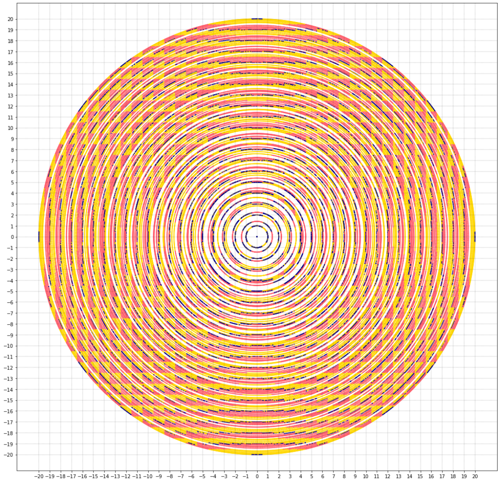
Here’s a simple dynamical system. You start with a 2D integer vector $v = (x,y)$ . Now you rotate this vector around the origin by a fixed angle. This gives you a vector $Mv$ (where $M$ is the rotation matrix). You now round this vector to the nearest integer lattice point, producing a new integer vector $[Mv]$ . You can repeat this process of rotation and rounding to produce $[M[Mv]], [M[M[Mv]]]$ and so on.
The 2D Rotation Rounding Problem is very easy to state: Does this sequence always end up repeating?

It doesn’t sound very hard, and if you change the question slightly, it becomes quite simple. If there was no rounding the answer is YES if the angle is a root of unity, and NO if it’s not (essentially by definition).

If we always rounded down (towards the origin), there’s only a finite number of integer vectors at the same or smaller distance from the origin and so by the pigeonhole principle , eventually you must repeat.

But by going to the nearest integer point we sometimes round up, and its juuust possible that – to quote Joel – “the planets align perfectly” and you keep getting to round up often enough to escape to infinity and beyond.

I tried testing a few examples.

Here’s an illustration of what happens with $v = (83,143)$ and angle $36 \pi /47$

Colors change from dark to light over time

It repeats at the 715th iteration.

In all the examples I tried, the sequence started to repeat within the first 1000 iterations. The authors of Reachability in dynamical systems with rounding never found a non-repeating sequence either, and they conjecture none exist.

The trouble is that large starting vectors are more likely to diverge to infinity (more options to avoid being pigeonholed), so running simulations for a finite number of starting points doesn’t confirm anything.

So the only way forward is to prove that all sequences repeat (or not). But how?

Points that get rounded up (yellow), down (red) or stay the same distance from the origin (blue).

Posted on September 25, 2020September 25, 2020 by Julian R. 0

How Come Deep Neural Networks Generalize?

This is a short review of the paper Understanding Deep Learning Requires Rethinking Generalization by Zhang et al, published in ICLR 2017, which I wrote as part of the application to the Google Research India AI Summer School.

The paper Understanding Deep Learning Requires Rethinking Generalization by Zhang et al, examines the question: Why do deep convolutional neural networks generalize well?

More precisely, models like AlexNet and its successors are able to achieve 70% test accuracy (90% considering top-5 guesses) on image classification using the CIFAR10 and ImageNet datasets.

In statistical learning theory, bounds on whether a hypothesis class can generalize to unseen data depend on whether it can shatter (informally, represent every possible input-output mapping) the training data. Intuitively, if the model can memorize the dataset it need not learn anything useful for unseen data. When dealing with highly expressive model classes, regularization methods (such as weight decay) are used to penalize expressivity and hopefully force the model to learn some kind of signal in the data, and not memorize.

Zhang et al show that this can’t be going on in deep conv nets, because these networks easily learn random labels to 100% train accuracy, even with regularization! They can indeed memorize random data, so regularisation is not doing its (theoretical) job of bounding expressivity. (One exception: AlexNet with both weight decay and data augmentation failed to converge on CIFAR10) Another point against the role of regularisation is that dropping it reduces test accuracy by only about 5%, so it’s not the main driver of generalisation ability.

Another hypothesis is that something about the structure of convolution neural networks makes it easy for them to learn images. (perhaps filters help pick out edges)

However, the authors show that conv nets easily learn images of Gaussian noise. It did take longer to learn random labels than random noise, which may indicate that some kind of forced declustering of natural clusters occurs.

The authors also find that regularisation seems to have benefits in optimization and prove a theorem showing that two layer ReLU networks can memorize n data points in d dimensions using 2n + d parameters. Note that the models used have about 1.5 million parameters, while ImageNet has 1.3 milion images (50000 for CIFAR10), so memorisation is certainly a plausible outcomes.

Thus we are still left with the question: How do we explain the impressive generalization ability of these models?

The authors analyse stochastic gradient descent in the context of linear models, and show that it finds the minimum-norm weights, which is promising, as it seems like SGD is implementing some kind of implicit l-2 regularisation. However, preprocesing the data leads to solutions with higher weight norms but better test accuracy.

Clearly, statistical learning theory cannot currently explain why deep (and large) models generalize well. So why do they?

One hypothesis (related to the manifold hypothesis) is that the test data simply isn’t that different from the training data, and these models are simply interpolating the test data based on the clusters they’ve learned. The models have enough parameters to disentangle the data manifolds of the various classes. (see Chris Olah’s post https://colah.github.io/posts/2014-03-NN-Manifolds-Topology) Of course, this still leaves us with the question of how these highly expressive models manage to find the correct manifold representation in the first place.

It’s also possible that there’s some overfitting going on. Madry et al’s recent paper From ImageNet to Image Classification: Contextualizing Progress on Benchmarks finds that roughly 20% of ImageNet images contain more than one object, making the correct annotation unclear. They note that for a third of all multi-object images the ImageNet label does not even match what new annotators deem to be the main object in the image. Yet, even in these cases, models still successfully predict the ImageNet label (instead of what humans consider to be the right label) for the image. This lends support to the theory that ImageNet images are very similar to each other. While considering top-5 accuracy helps alleviate issues with multi-object images, it leads us to overestimate accuracy on single-object images.

To conclude, it’s interesting that this paper was written in 2016, and as far as I can tell we still don’t really know why deep conv nets generalize! I’m pretty optimistic that rapid improvements in visualization methods will help us see what’s going on more clearly.

Posted on July 9, 2020July 9, 2020 by Julian R. 0

Qubits and the Kernel Trick: The power of working in a bigger space

I’ve been reading Mermin’s account of Deutsch’s Problem, and it’s given me a new insight into where the power of quantum computing comes from.

If you look at the original problem, you have a function f(x) from {0,1} to {0,1}. There are 4 such functions.

Function	f(0)	f(1)
f_1	0	0
f_2	0	1
f_3	1	0
f_4	1	1

The four distinct functions from 0,1 to 0,1

What can you learn by calling the function once? If you call it with 0 as input, you separate 1,2 from 3,4. By calling f(1) you separate 1,3 from 2,4.

Can you separate 1,4 from 2,3? In other words, can you answer the question “Does f(0) equal f(1)?” with a single function call? It’s impossible: Classically! (Try it and see)

In classical computing you have some bits and the only thing you can do to them is flip em from 0 to 1 and back and permute them around.

Quantum bits have additional properties. They can be rotated! More precisely, if you consider 0 and 1 to be two orthonormal vectors in a 2-dimensional complex vector space, quantum bits can be any unit vector in that space. The idea of a complex linear combination (of the computational basis vectors 0 and 1) is something that makes no sense in classical terms. Yet we can do operations with those combinations, rotate back into one of the classical bits, and get out a classical answer. Deutsch’s algorithm (explained on Wikipedia) uses Hadamard gates, which let you apply the function f (once!) to the qubit represented by $(\frac{|0\rangle}{\sqrt{2}} + \frac{|1\rangle}{\sqrt{2}})$ . After some more hadamard gates you get to measure a bit which is 1 if f(0) equals f(1) and 0 otherwise. Note that you do not get to know either f(0) or f(1), so you haven’t magically gained more information from your single function call, just different information which you could think of as “perpendicular” to the classical way of seeing things.

I just realised that there is something which forms a useful analogy for the power of quantum computing: the kernel trick in SVMs!

Support vector machines work by taking dot products of data vectors with special vectors called support vectors. We might have some data which may not be linearly separable in the space we’re working in, but might be separable in a higher dimensional space. In other words, there might be some fancy function $\phi$ such that working with $\phi (x) \cdot \phi (y)$ lets us linearly separate things even though $x \cdot y$ doesn’t work. The kernel trick is that we can actually compute $\phi (x) \cdot \phi (y)$ from $x \cdot y$ without having to compute $\phi(x)$ or even work in the high-dimensional $\phi$ -space at all. So what we do is we take the dot product $x \cdot y$ (linear), and compute some nonlinear function of it (say we take the square). Magically, this function turns out to be the dot product of $\phi (x) \cdot \phi (y)$ for some function $\phi$ !

Of course, the caveat is that you can’t get just any function this way, but in practice you’ll easily find some function which lets you separate the data.

To work through an example of what I described above: Let $x = (x_1, x_2)$ . Then $x \cdot y = x_1y_1 + x_2y_2$ . Suppose our kernel function was $K(x,y) = (x \cdot y)^2$ . Then we get $K(x,y) = (x_1y_1 + x_2y_2)^2 = x_1^2y_1^2 + 2x_1x_2y_1y_2 + x_2^2y_2^2$ ,which can be written as $(x_1^2,\sqrt{2}x_1x_2,x_2^2) \cdot (y_1^2,\sqrt{2}y_1y_2,y_2^2)$ . But this is equal to $\phi (x) \cdot \phi (y)$ , where $\phi$ is the non-linear function $\phi (x_1,x_2) = (x_1^2, \sqrt{2}x_1x_2, x_2^2)$ !

So using kernel functions, by sacrificing other information to only learn about dot products, we’ve managed to leverage the power of computing in the $\phi$ -space, without actually needing to explicitly compute $\phi (x)$ .

Analogously in quantum computing, interference among complex linear combinations of classical bits let us compute (classical) answers to questions that cannot be answered using only classical operations. Note that we do not (and cannot) get “other” information like the complex coefficients of the qubit.

Because every good analogy deserves a table of correspondences

\phi (x) — Because every good analogy deserves a table of correspondences

Posted on June 10, 2020 by Julian R. 0

Book Review: T. Tembarom by Frances Hodgson Burnett

Frances Hodgson Burnett (henceforth FHB) is well known as the author of The Little Princess and The Secret Garden, which are books I vaguely remember as classics from my childhood though I cannot swear to having actually read them. It turns out she was a bestselling author in her day, and wrote at least twenty other books, including the interestingly titled T. Tembarom, published in 1910.

I decided to read it solely because of the description in AJ Hall’s review.

The book starts with a philosophical argument that our sources of information about the world are skewed away from learning about most people, who are fairly nice and good, as is the nature of human beings, if there isn’t something aberrant about them.

No one has ever made a collection of statistics regarding the enormous number of perfectly sane, kind, friendly, decent creatures who form a large proportion of any mass of human beings anywhere and everywhere—people who are not vicious or cruel or depraved, not as a result of continual self-control, but simply because they do not want to be, because it is more natural and agreeable to be exactly the opposite things; […] When one reads a daily newspaper filled with dramatic elaborations of crimes and unpleasantness, one sometimes wishes attention might be called to them—to their numbers, to their decencies, to their normal lack of any desire to do violence and their equally normal disposition to lend a hand. […] They really form the majority; if they did not, the people of the earth would have eaten one another alive centuries ago. But though this is surely true, a happy cynicism totally disbelieves in their existence. When a combination of circumstances sufficiently dramatic brings one of them into prominence, he is either called an angel or a fool. He is neither. He is only a human creature who is normal. After this manner Tembarom was wholly normal.

FHB seems to imply that most people are like T. Tembarom, but if there is one thing that the story makes clear, it is that T. Tembarom is most certainly not normal.

T. T. (as his friends call him) is blessed with almost superhuman good cheer, bounding energy, and a near complete inability to feel sorry for himself. Scarcely less unusual is the story’s other protagonist, Little Ann Hutchinson. They are both without flaw and never put a foot wrong throughout the book. If this was a modern novel, would I have thrown the book against the wall for their sheer Mary Sue-ness?

To illustrate, I can’t do better than quote A J Hall’s description of how the book starts (from the review I mentioned) :

T.Tembarom is the preferred name of the hero, whom we first meet at the age of ten, when, his mother having just died in a New York tenement, he spends his last cents, and twenty more cents he borrows from a neighbour on buying some newspapers to sell. After this, by dint of hard work, undaunted good humour, nightschool shorthand, apparent imperviousness to hypothermia and general applied niceness he works his way up to his a lucky break, namely the opportunity write a Society column on a Sunday paper, whose circulation appears to be predominantly in the Bronx, at the princely sum of $25 per week.

The only problem is that he doesn’t have a clue (a) how to gather material for the column; and (b) how to write it up once he’s got it.

In this dilemma he turns to “Little Ann” Hutchinson, who is living in the same boarding house as him, along with her father, who is a disillusioned inventor from Lancashire.

[…]

Every young man in the boarding house is in love with Little Ann, who darns everyone’s socks, mainly I think to give her hands something to do while her formidable intellect and talent for headology is clicking into gear.

Little Ann’s sensible suggestion is to start gathering material for Society weddings with the wedding caterers. T.Tembaron runs with this suggestion, even though there’s a blizzard going. Little Ann does not say, “Do not go out into the blizzard scraping acquaintances with wedding caterers.” Little Ann lends him her father’s muffler and tells him to make sure he gets the names of the dress fabrics right. T.Tembaron, having made a huge hit with the caterers, befriends a dressmaker and gets samples so he can learn them by heart and spot them at sight. And when his first attempt at the column is rejected by his editor on the basis that it’s full of purple prose Tembarom has plagiarised out of other newspaper columns and his $25 per hangs by a thread, she ruthlessly sub-edits him, too.

The course of true love running moderately well, and T.Tembaron starting to look hopefully at advertisements for small flats in high rise buildings in the newly built upper 140s and lower 150s, he is devastated by twin blows: first, Mr Hutchinson’s pitch of disillusionment has now become so elevated that only a return to Lancashire will assuage it, and Little Ann will, of course, dutifully accompany him, and, secondly, at the ‘oyster stew’ thrown by way of farewell party to them at the boarding house, a very stuffy London lawyer shows up and reveals T.Tembarom’s real name (and since it’s Temple Temple Barholm, you can see why he’s concealed it for the last quarter of the book) and announces that he’s — ta da! — the missing heir to the village and estates of Temple Barholm, in Lancashire. At which point Mr Hutchinson is struck all of a massive heap and confesses that he was born in that very village! And he learned his letters at the village school! And his aged mother lives in a cottage there still!

And Ann, very sensibly, says no, she isn’t going to marry T.Tembaron straight off, nor is she going to put up with his cancelling their steerage passages for tomorrow and booking them first class staterooms so they can travel along with him in three weeks time: he’s got to get used to being Temple Barholm of Temple Barholm, lord of the manor with £70K per annum, and see all the Society beauties whom he is now eligible to marry, and when he’s had a year of that she’ll think about it.

And from then on the plot moves to Lancashire and more shenanigans ensue.

I found the book paradoxically very slow to read but entertaining. The kind of book that is supposed to be your sole entertainment for the entire week. And this appears to be a linear function of age, since I once tried reading The Woodlanders by Thomas Hardy, and that was clearly supposed to occupy you for a month. It took me weeks to read the first half of T. Tembarom, but sometime ago I was stuck on a train with nothing else to do (as God and FHB intended) and the second half was quite the page-turner.

The best part of the book was how inspired I was by T. Tembarom’s unflagging determination and even less flaggable good cheer. The man spends significant portions of the book trudging through blizzards and being icily snubbed by high society beauties. And while he might not be grinning at those particular times (he spends most of the book with an ‘extraordinarily friendly grin’), he sure as heck doesn’t let them get him down either.

The other thing I got out of it was a renewed appreciation for how lucky I am to be born in the 21st century. Nearly all the choices I have right now in terms of career options and people I could talk to are more interesting than those available to a character who is a literal duke.

Something that really stands out is how the position of women in society has changed. There are two characters, upper-class women who see no possible future before them apart from making a rich marriage and starving in genteel poverty. However, it’s hard to tell how much of this is the British upper-class refusal to stoop to ‘trade’.

I was far more frustrated by Little Ann Hutchinson’s attitude to her father and FHB’s implicit approval of her attitude.
The man is utterly without the slightest shred of self-awareness and humility. Little Ann spends half the book carefully steering him out of the clutches of various conmen and massaging his male ego. While Mr Hutchinson bloviates about the native shrewdness of Lancashire folk and how “women are not up to much at business”, Little Ann, under the guise of “I am but a girl and know nothing of business of men’s affairs”, exclaims about how adroitly he handles all the speculators that come to them and how clever he must be to find the loopholes in their proposal. Quickly enough Mr. Hutchinson begins to think that it was actually him who figured out all the holes in the conmen’s stories, and talks with extreme condescension towards little Ann. In Little Ann’s place I would started punching walls. On the other hand, I’m not sure how I feel about the way Ann treats her father’s character as an obstacle to be worked around. Why not be a bit more direct? It feels a little manipulative, though it’s very clear she loves him, and wants him to be happy and keep his illusions unshattered (while making sure they don’t get scammed).
While I’m not sure I could do it, it seems as if, given the constraints of her time and place in society, little Ann behaves in the way that is optimal for achieving all her varied goals.
I suppose I give the man some credit for realizing how much better things go when Ann’s around, and making sure she’s always with him when embarking on a new business transaction.

While the book was published in 1910, it feels like it’s describing a much older time, and indeed the mention of President Garfield’s assassination puts the story in the 1880s.

Would I recommend this book?
Tough to say. I certainly don’t regret reading it, and I intend to continue singing the phrase ‘T. Tembar-om-om’ to the tune of the hymn ‘Here I Am, Lord’, anytime I need to be reminded of the power of approaching life with an “extraordinarily friendly grin”.

I did, however, approach it in exactly the right spirit, (thanks to A J Hall) prepared to look past FHB’s insane Victorian morality and style to find the good parts.

It’s always an interesting exercise to read old books, since even if the plot isn’t very compelling, you can always turn it into an anthropological study of the author’s milieu.

If you can stand the pace, and T. T. thinking about how he wants to embrace little Ann for the hundredth time, T. Tembarom‘s free on Gutenberg – have fun!

Posted on April 22, 2020June 10, 2020 by Julian R. 0

	Anish Kumar on Poisoned Cookies
	Julian R. on Poisoned Cookies
	How much kale is con… on Poisoned Cookies
	chiqutam on Poisoned Cookies

Kernel Trick	Quantum Computing
$x$	Classical bit ( 0 or 1)
$\phi (x)$	Qubit in quantum superposition ( $(\frac{\|0\rangle}{\sqrt{2}} + \frac{\|1\rangle}{\sqrt{2}})$ )
$\phi (x) \cdot \phi (y)$	Classical indicator function $1_{[f(0)=f(1)]}$
$K(x,y)$	Quantum circuit

just unreadable icon